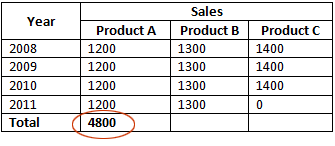
Microsoft Word lets us do some calculations on tabular data. In this tutorial, I shall show you how to calculate the sum of the values of a column. I have tabular data like the following table.
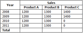
To calculate the sum for the “Product A” column, place the cursor at the last cell of column 2 (cell marked in yellow color).
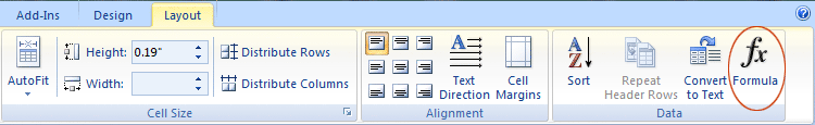
Press the “Formula” button (marked in the red circle).
A “Formula” dialog box will appear.
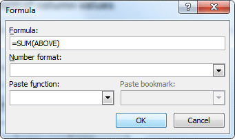
There are some options we can choose from here.
We shall write a formula in the “Formula” text box. I have used the following formula:
=SUM(ABOVE)
It will calculate the sum of the values of the upper cells.
In the “Number format” combo box, there are options to control how we can format the number.
In the “Paste function” combo box, MS Word has listed some predefined functions. We can choose any item from the list to take into our account while calculating the formula.
Now press the “OK” button.
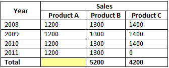
You get the total for the “Product A” column. Repeat these steps to calculate the sum for other columns.
Caution
Make sure that there is no empty cell in any cell of the column, or you won’t get the correct result. Put a “Zero” (0) in the cells whose values are empty.
Leave Your Comment